I built a Twitter analytics service. Most of the work was figuring out why it was slow.

By Phase 3, I had a Twitter analytics service handling 20,000 requests per second on ECS Fargate and RDS at $0.31 an hour. My Phase 1 result had been 353.25 requests per second. A separate Redis-only experiment pushed throughput to 70,000 requests per second by keeping the data in memory, but it was expensive.

That is the tidy version. It skips the hours spent rerunning ETL, the database imports that took another three hours, the memory setting that stopped MySQL from starting, and the deployment that looked fine until the application tried to connect to its database.

The less tidy version is more useful.

Before the service, learning to work with the graph

The semester project began with a different Twitter dataset: a 10.4 GB follower graph. Before I had an HTTP service to optimize, I had to learn what Spark was doing with hundreds of millions of relationships. The recorded analysis found 1,006,458 vertices and 564,768,812 directed edges.

I wrote the follower-count calculation twice. In the RDD version, I mapped each edge to a followee and a count, then used reduceByKey so Spark could combine counts within a partition before shuffling them. The DataFrame version expressed the same problem as an aggregation, sort and limit, then wrote the result as Parquet. That let me compare two ways of describing the work instead of hiding one API behind the other.

PageRank introduced repeated computation. The graph stayed fixed while each user's rank changed, so I computed and cached the adjacency and out-degree information once. Each iteration joined that static data with the current ranks. I also had to account for dangling nodes: rank mass could not simply disappear when a vertex had no outgoing contribution.

The retained implementation handles PageRank and dangling mass; the bonus recommendation aggregation still has an unfinished section. The separate graph-analysis answer file is complete. I do not have a final runtime proving the under-thirty-minute performance target or evidence that the Databricks bonus was finished.

That preparatory phase shaped the later service. I started looking for work that could be done once, stored, and reused. When the tweet dataset arrived, that became the central design decision in the ETL pipeline and the database schema.

The request and the constraints

I built this for the Spring 2026 cloud computing semester project, from February through April: first getting the service correct, then making it fast, then moving it onto managed AWS services. Along the way, I changed where the work happened, how the data was stored, and how much infrastructure I actually needed.

The service answered a specific question. Given a Twitter user, an interaction type such as replies or retweets, a phrase, and a hashtag, it ranked that user's contacts using their interactions and the supplied search terms. The response included user information and the latest relevant contact tweet. Each request also needed a token from the provided authentication service.

The challenge was to turn a supplied historical dataset of messy tweets into something I could query correctly, repeatedly, and cheaply, following a prescribed scoring and response format.

I started with Java because I knew Java. There is no more impressive explanation hiding behind that decision. I used Java 17, its HTTP server, Maven, JUnit, and Docker. The tests came before the initial server implementation. First I got requests and authentication working; the analytics logic came later.

For authentication, I chose REST. The interaction was a small JSON request and response, and it was easy to inspect when something went wrong. I considered gRPC, but I did not implement and benchmark both protocols. Once I had caching and duplicate-request suppression, I had other bottlenecks that deserved more attention.

The first cloud setup used a self-managed Kubernetes cluster with kOps: one m6g.medium control-plane node and two m6g.medium workers. An Application Load Balancer (ALB) routed public traffic to Twitter; authentication and MySQL were separate internal services.

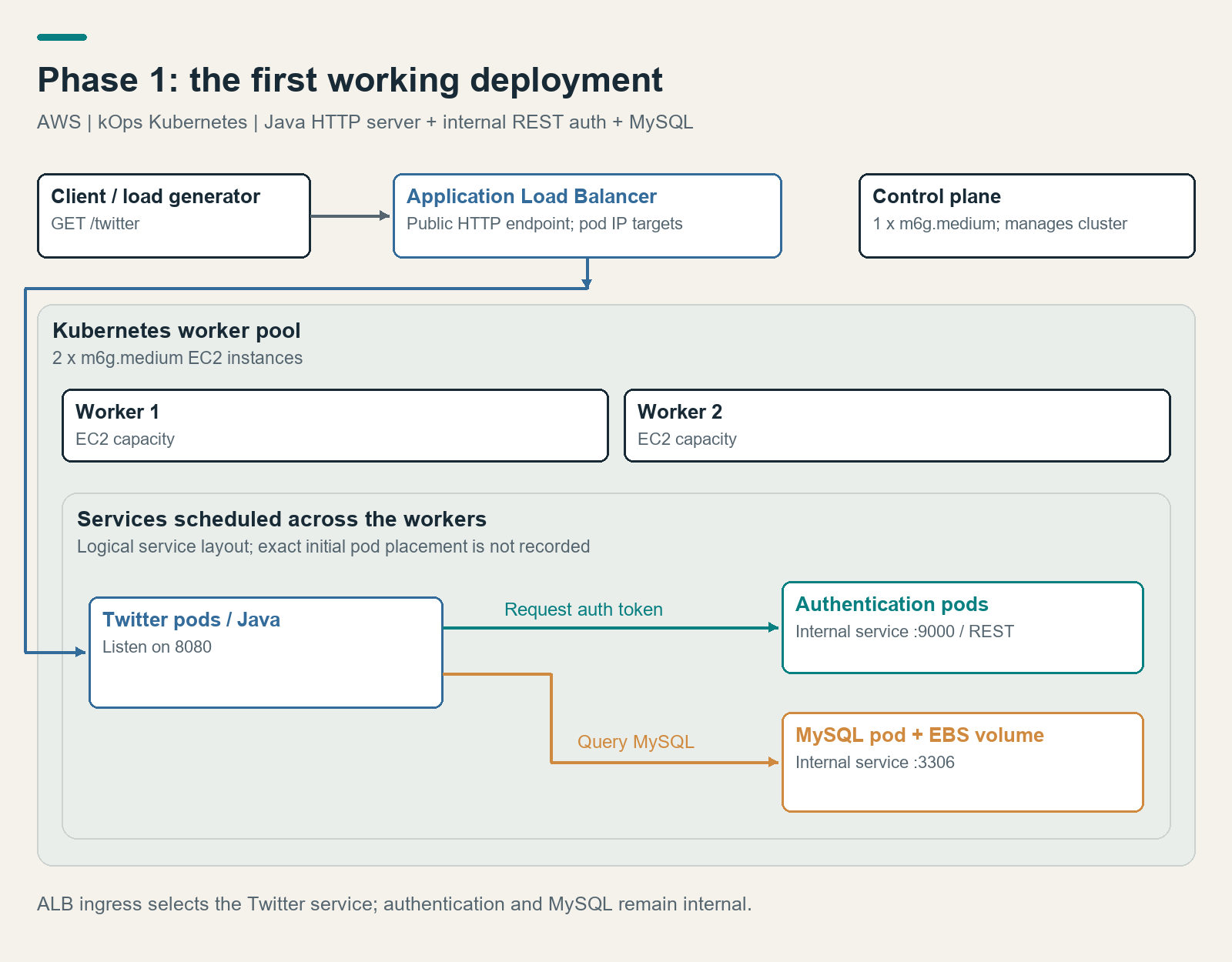
Separate services let me scale Twitter and authentication independently. But pods on the same worker still shared CPU and memory. Their placement would become much more important later.

Phase 1 had a $0.27-per-hour constraint and emphasized correctness. At that point, buying more capacity would not have fixed a wrong score or a badly formatted response. I needed the whole request path to work before I could sensibly optimize it.

Making a terabyte queryable

Then there was the data.

The input was about one terabyte of raw Twitter data. I wrote the ETL pipeline in Scala and Spark using Zeppelin, initially running locally through Docker. Scala was something I had recently learned, and the notebook let me inspect intermediate results. I used MySQL Workbench to explore the data and try queries.

My laptop could handle tests on a handful of files. It could not comfortably stand in for the full dataset. For the full ETL run, I moved to GCP, using one n2-standard-4 master and five n2-standard-2 workers.

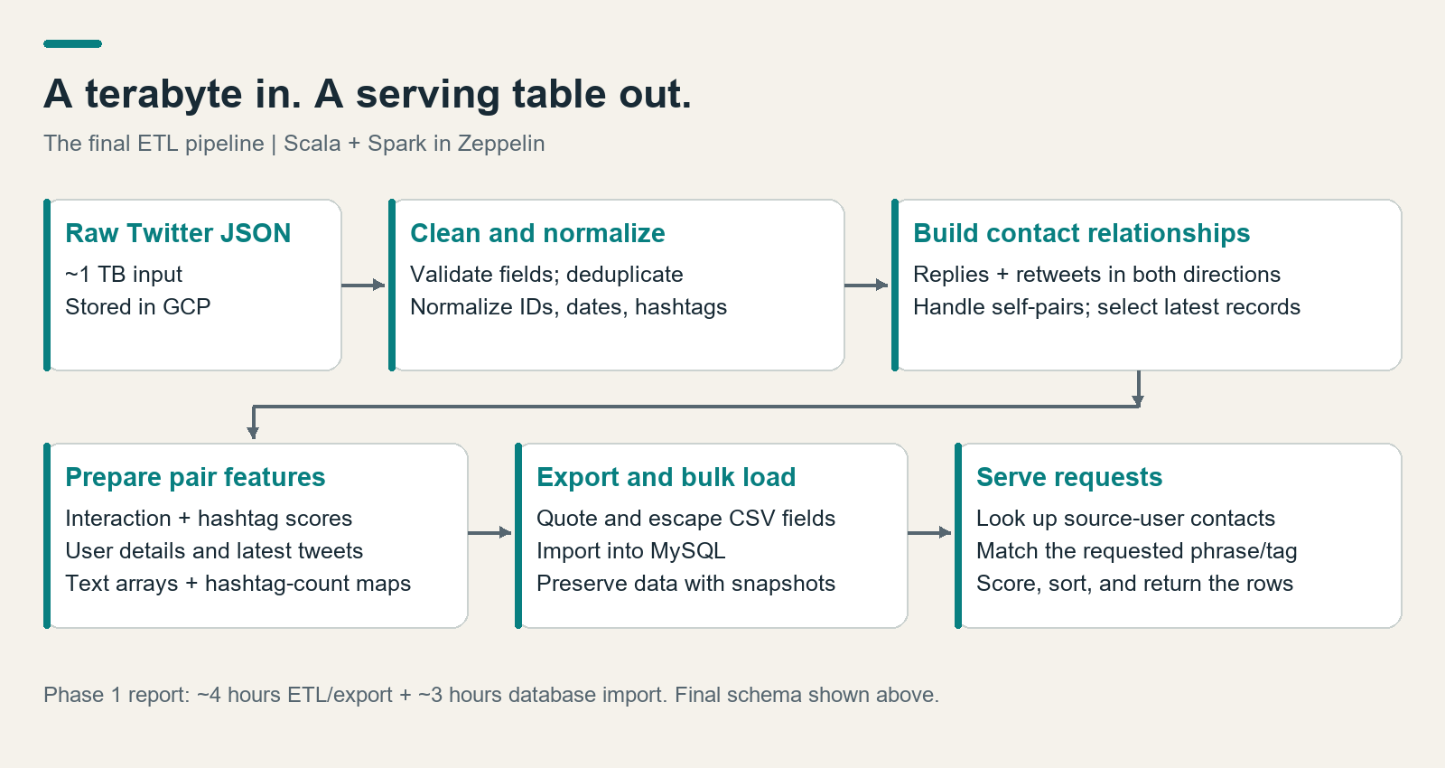
The cleaning rules mattered as much as the aggregation. I filtered malformed or incomplete records, checked the required fields and allowed languages, normalized IDs that could arrive as numbers or strings, parsed timestamps, and deduplicated tweets. Hashtags needed consistent casing. Replies and retweets became contact relationships between users.

I stored relationships in both directions so a lookup could start from either user. That meant handling self-interactions carefully: blindly reversing a self-reply would count the same interaction twice. For the latest tweet and user information, I used timestamp ordering with tweet IDs to break ties. These sound like small details until one of them changes the final ranking.

Spark also calculated interaction scores and shared-hashtag features. The interaction score weighted replies more heavily than retweets. For the shared-hashtag calculation, I excluded the supplied list of popular hashtags. The pipeline kept separate contact hashtag counts for matching the hashtag in an incoming request; those were a different part of the scoring logic.

The first report records around four hours for ETL, including export, followed by about three hours loading MySQL. The reported ETL cost was $22.91. Exporting the CSVs consumed a large part of the processing time. The processed export was roughly 23 GB, while the database was around 80 GB in that phase. Storing bidirectional relationships to reduce query work was one reason I accepted a larger database.

And I had to do parts of this more than once.

My local tests were useful, but insufficient. Some problems only became visible against the larger dataset. The commit history has a whole little trail of delimiter changes, sanitization corrections, and line-ending fixes. Tweet text is not polite tabular data. It contains quotes, tabs, and newlines, and those characters have to survive Spark export, database import, and response formatting with the intended meaning.

I revised the intermediate-storage approach too. One early ETL commit explicitly removed Parquet intermediates to improve speed. The later notebook persisted selected intermediate datasets to disk to reduce memory pressure and avoid recomputation. These were practical changes to this pipeline, driven by where it was spending time and memory.

The lesson was expensive in a very literal sense: a bug near the end of a pipeline can make you pay for the beginning again. Next time, I would test more representative edge cases and extract the transformations into reusable Scala code. Keeping separate test snippets synchronized with notebook paragraphs was asking for trouble.

I bulk-loaded MySQL with LOAD DATA INFILE and LOAD DATA LOCAL INFILE, then took EBS snapshots. Creating one took roughly 45–60 minutes, but restoring it avoided another three-hour import. I needed a second snapshot after finding issues in the first dataset. A snapshot is very good at preserving whatever you give it, including your mistakes.

Five queries became one

My first database design spread the data across five tables: latest_user_info, contact_tweets, latest_contact_tweet, contact_tweet_hashtags, and pair_features. I had already precomputed some scores, but the service still needed several lookups to assemble a response.

It was understandable when I looked at the schema. Under load, it was painful.

Some of the larger requests needed five sequential queries and took up to three seconds. I could adjust connection pools and add pods, but every uncached request still had to walk through that sequence. I was repeatedly reconstructing information that barely changed.

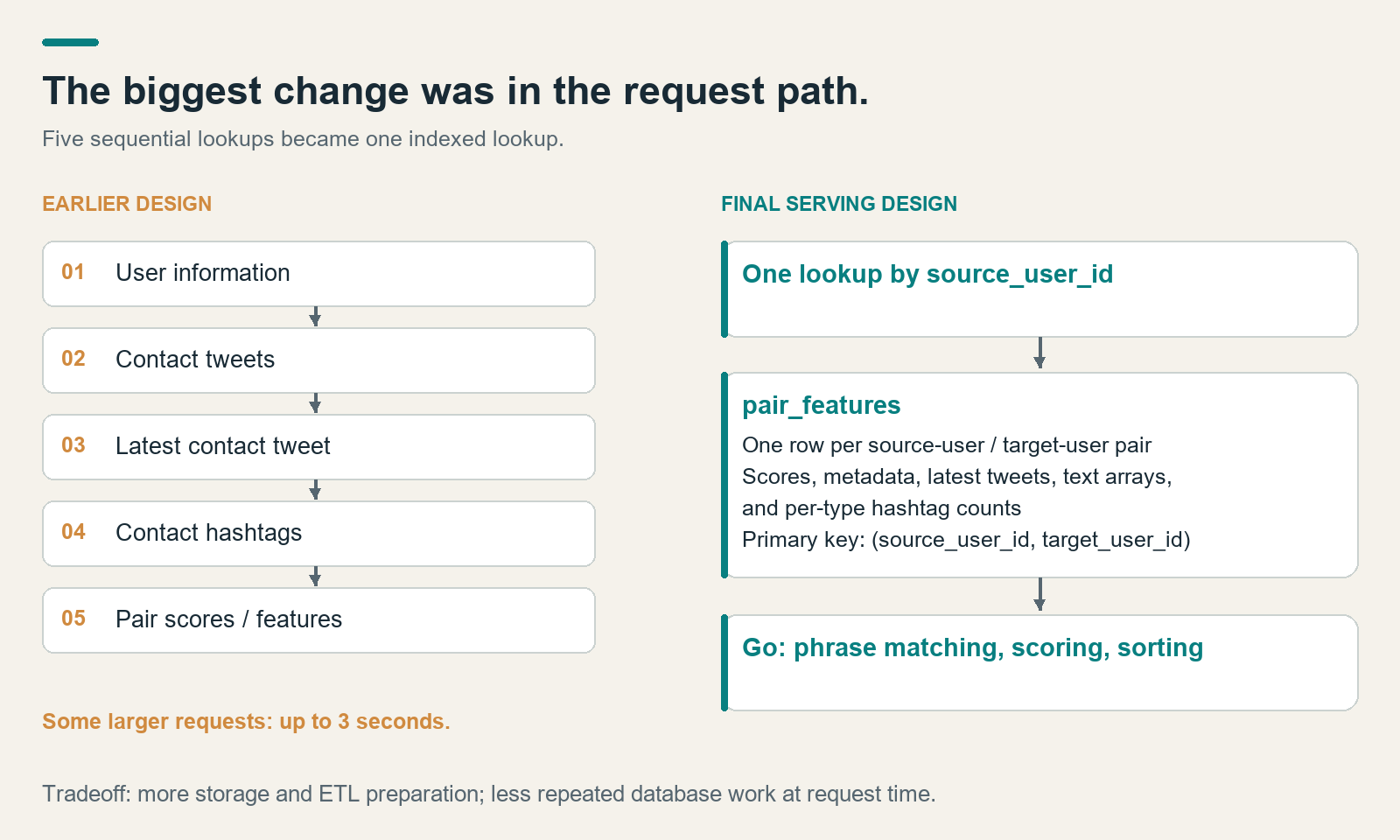
In Phase 2, I collapsed the serving schema into a single, denormalized pair_features table. Each row represented a source-user and target-user pair. Alongside precomputed scores and counts, it held the target user's metadata, the latest reply and retweet text, the latest contact tweet across both types, hashtag-count maps, and arrays of tweet text.

The primary key was (source_user_id, target_user_id), which supported the service's lookup by source user. I accepted duplication because this workload was overwhelmingly reads over a fixed dataset. I could pay for more preparation and storage once, then do less database work on every request.

There was still real computation left in the application. The phrase in the query was only known when the request arrived, so I could not precompute every final answer. The service loaded the relevant pair features, counted phrase and hashtag matches, combined those with the stored scores, rounded the result, sorted the contacts, and rendered the response.

I also followed through on the Go rewrite I had been considering since Phase 1. The first Go Fiber implementation appears in early April, followed by the version that used the denormalized database. I kept the Java implementation in the repository for reference and testing.

The rewrite helped: my report records roughly a 30% improvement, from about 1,000 to 1,300 RPS. But crediting the final result to Go would be overselling it. The denormalized setup eventually reached roughly 5,500 RPS after further optimization. These were evolving configurations, not a controlled language benchmark. Removing repeated database work was the larger architectural change.

The Go service also got two bounded, in-process LRU caches: one for authentication tokens, keyed by timestamp, and one for query results, keyed by user, interaction type, phrase, and hashtag. The final code gives them capacities of 4,096 and 2,048 entries respectively.

Caching only solves the repeated request after the first result exists. If several identical requests arrive together and all see a miss, they can still produce several identical database calls. I used singleflight to let concurrent requests for the same work share one in-flight computation. I applied that to both token requests and data queries.

I reused HTTP connections, bounded database connection pools, and timed authentication, database loading, ranking, and rendering. Tests covered overlapping phrase matches, rounding, tie-breaking, JSON decoding, and multiline output. Chasing throughput did not make those correctness details go away.

The caches were local to each process, lost on restart, and capacity-limited without time-based expiration. That fit this fixed-data project more comfortably than changing tweets or different token-validity rules. Those assumptions would need another look before reusing the design.

I also alternated reads between two MySQL instances, each with its own data volume. This distributed the workload across two copies of the data. The round-robin code did not provide health-aware failover, so the extra capacity should not be confused with a complete high-availability system.

Finding the next bottleneck

After denormalization, the metrics started telling a different story. At one point, the database nodes were around 40–45% CPU while the web nodes were close to 100%. The database could return the data quickly enough that the application tier was now the limiting factor.

That led to one of the more satisfying changes in the project. My final Phase 2 cluster had one m6g.medium control-plane node and four m8g.medium workers. Two workers each ran two Twitter pods. The other two each ran MySQL, authentication, and one additional Twitter pod. That gave me six Twitter pods, two auth pods, and two MySQL pods.

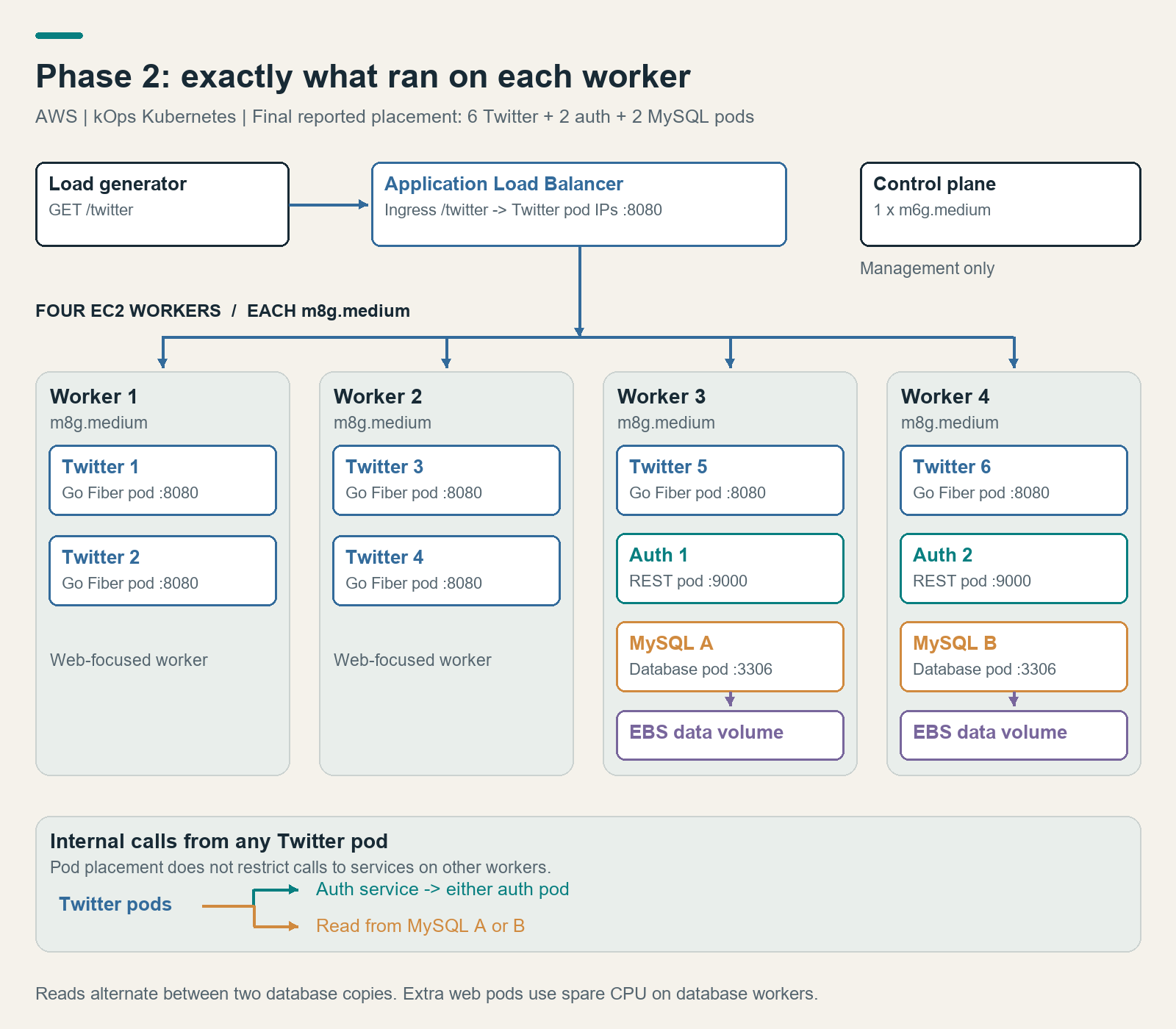
I used affinity and anti-affinity rules to guide that placement. Putting an extra Twitter pod on each database worker let me use CPU that the optimized database no longer needed. The report compares around 4,000 RPS with the more strictly separated layout against roughly 5,500 with those extra application pods.

I tuned pod limits, replicas, connection pools, and InnoDB memory. The git history has the kind of commit messages that happen when you are chasing a number: eight pods and 547 throughput, then ten pods and 702. Those were early steps toward the final result.

My buffer-pool experiment was especially blunt. The report records approximately 4,000 RPS with a 1 GB buffer, 5,500 with 2 GB, and a failed startup with 3 GB. I had given the cache too much of the machine's memory. MySQL and Kubernetes still needed room to exist.

A larger cache sounds good right up until the service cannot start.

I experimented with CPU limits above a worker's nominal capacity after observing underutilization. That did not create CPU; it relaxed limits while accepting more contention. I was squeezing a small cluster fairly hard.

During the Phase 2 live test, I watched CloudWatch and Headlamp, checked pod placement and restarts, and kept an eye on memory. The run went smoothly. The database workers came close to using all their memory, which was exactly the part I had been worried about.

The final Phase 2 performance run reached 5,516.19 RPS, about 15.6 times the Phase 1 result. The reported hourly cost was $0.3753 under the project's accounting rules. It was a much better service, but it still needed me to manage the cluster and the database containers.

Moving to managed services

Phase 3 changed the infrastructure question. I had to use managed services, and the performance-to-cost ratio mattered. I explored ECS with Fargate and EKS with Fargate, and costed an EKS managed-node alternative. I did not complete a comparable performance experiment for every architecture.

I chose ECS Fargate for the final performance deployment. The application was straightforward enough that ECS services and task definitions covered what I needed. In the project's cost model, the EKS control-plane fee alone was about $0.10 an hour. Against the $0.31-an-hour Phase 3 result, that was a substantial amount of budget before adding application capacity.

The final deployment put an internet-facing Network Load Balancer in front of the Twitter tasks. The auth service was discovered through private DNS, and the database became a private, Single-AZ RDS MySQL instance. Terraform described the infrastructure, including the services, task definitions, networking rules, load balancer, and logging. The task definitions used ARM64 images, and database credentials came through AWS Secrets Manager.

I restored RDS from a snapshot for repeatable setup. The older EBS snapshots needed a different migration path: recover self-managed MySQL, then transfer the data into RDS.

Managed services reduced the amount of infrastructure I had to babysit. They still left plenty of ways for components to fail to talk to each other.

The application deployed but timed out reaching MySQL because RDS's security group did not allow traffic from the web tier. Allowing port 3306 from the correct security group fixed it. In EKS, this connectivity problem showed up as a Twitter pod repeatedly crashing and restarting.

An old affinity rule also prevented an authentication pod from scheduling in the new cluster. I added CI/CD-specific Helm values and removed the outdated requirement. A rule that helped the previous deployment was breaking this one.

These were not especially glamorous fixes. Reading the logs, inspecting the pod, and checking the actual network permission got me further than staring at an architecture diagram.

The biggest Phase 3 performance lesson came from database warm-up. I initially saw around 6,000 RPS with a larger application deployment. Repeated runs with the same configuration improved, and the utilization pattern changed as useful database pages became resident in memory. I had been treating the first run as more representative than it was.

Once I understood that behavior, I could make a better decision about task counts. I scaled down and watched whether the remaining tasks could still handle the workload. One configuration documented in my report used two Twitter tasks, each with 1 vCPU and 2 GB of memory, and two authentication tasks, each with 0.25 vCPU and 0.5 GB of memory. The report lists a db.r6g.large RDS instance with 120 GB of gp3 storage.

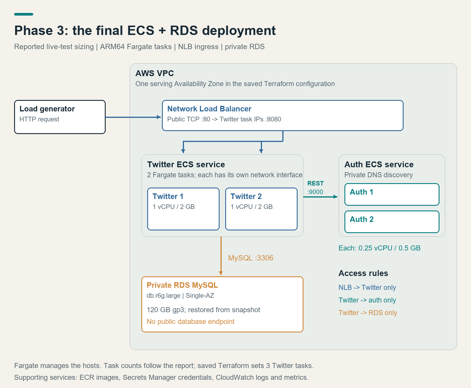
The Phase 3 result I achieved was 20,000 RPS at $0.31 an hour. The saved Terraform specifies three Twitter tasks, while the report describes a two-task configuration; those artifacts capture different points in the tuning process rather than one exact snapshot of every performance run.

Warm-up and the earlier optimizations let fewer tasks handle more traffic. Scaling down by itself was not a performance trick.

Reaching 20,000 requests per second

Getting to 20,000 requests per second was the combined result of the work that came before it: removing repeated database queries, precomputing reusable features, changing the web tier, and measuring how the deployment behaved under load. The cost mattered alongside the throughput. At $0.31 an hour, the Phase 3 configuration gave me a result I could defend on both measures.

I also wanted to see how far I could push the service with a different storage approach. That led to the Redis-only experiment below. Its higher throughput came with a different cost profile, so I keep it separate from the Phase 3 result in the graphic.

Pushing further with Redis and data in memory

For the experiment, I used Redis as the only serving data store and kept the data in memory, without a separate MySQL database in the request path. This went beyond caching a few repeated requests: the data needed to serve the workload was held in memory.

That version reached 70,000 requests per second. It showed what was possible when I changed the storage approach, but the configuration was expensive. I did not achieve that throughput at the Phase 3 cost of $0.31 an hour.

I would describe it as an experiment in throughput rather than the economical configuration I settled on. The exact hourly cost was not recorded here, and it was a different setup rather than a controlled comparison with the database-backed version. The useful lesson was to keep asking what I was optimizing for: the highest request rate, or a service that delivered strong performance within the budget.

What the numbers leave out

Automation grew alongside the application. I started with build-and-test and Helm lint jobs. I added image publishing to ECR, deployment workflows, and manual triggers so I could rerun a deployment without making an empty commit just to wake up the pipeline.

By the final phase, Java tests, Go tests, and Helm linting ran independently. A separate workflow published the Go image. The EKS workflow prepared cluster access and secrets, deployed routing and Helm releases, waited for readiness, and checked the endpoint. I kept EKS for the CI/CD requirement while using ECS for the performance deployment.

That endpoint check needs strengthening. It accepts HTTP 200, but the service also returns 200 with an INVALID body, and the test omits the required timestamp. I would verify a valid request and its response body before calling it deployment validation. The automation improved, but some checks were narrower than their names suggested.

There were experiments I left on the table too. I did not run a full ALB-versus-NLB comparison in Phase 2. Redis and Memcached were prohibited in that phase, which is why its caches lived inside the Go service. I kept MySQL for the managed Phase 3 configuration and explored Redis separately in the in-memory experiment.

The final system made a reliability tradeoff. Multiple tasks gave the web tier some resilience while ECS replaced failures, but Single-AZ RDS remained a critical dependency. It fit the budget. Running successfully during a test did not erase that risk or give a nearly saturated system much spare capacity.

If I built this again, I would start with a more representative ETL test dataset, put the transformations somewhere easier to test, and record performance runs with warm-up state, exact configuration, and latency distributions. I would preserve the configuration used for each reported result, validate real responses in CI, and make the cache freshness and database-failure behavior explicit.

What I am happiest with is the change in how I approached performance. Early on, I was adjusting threads, pods, and buffer sizes around a request path that did too much work. Later, I could point to the expensive part, change it, and then watch the bottleneck move somewhere else.

The part I would want another engineer to remember is simple: five sequential queries became one lookup, the database stopped being the slowest part, and that gave me a different set of decisions to make.

The two results capture that tradeoff: 20,000 RPS at $0.31 an hour in Phase 3, and 70,000 RPS in an expensive Redis-only experiment. The work underneath them was learning to make decisions with evidence, including when the evidence said my previous decision was wrong.